Discrete Time Signal Processing: A Primer

Discrete time signals are represented as a sequence of numbers. Say $x$ represents a sequence of numbers, then we may use $x[n]$ to denote the $n^{th}$ element in the sequence $x$. Here, $n$ is an integer. In practical terms, this representation could arise from periodic sampling of a continuous time signal. Each number in the sequence corresponds to a sample obtained at a sampling interval.

A visualisation of a discrete time signal $x[n]$ is illustrated below.

%matplotlib inline 
import numpy as np
import matplotlib.pyplot as plt

t = np.arange(0,0.2,0.01); # Sampling time instants
x = np.sin(2*np.pi*10*t);

plt.stem(x)
plt.xlabel('Sample Index - n')
plt.ylabel('Sample Value - x[n]')

plt.show()

png

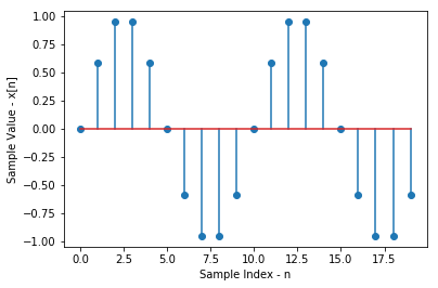
The above example shows a discrete time sine signal of 20 samples. This could be interpreted as samples of a continuous time sine signal at every $0.01$ seconds.

Most of the concepts that apply to continous time signals intuitively extend to discrete time signals. The reader is urged to draw analogies to aid in understanding. There are however, major differences as well. For example, one can delay a discrete time signal only by an integer number of samples. Another example is the fact that a discrete time periodic signal mandates that the time period be an integer multiple of the sampling time.

Discrete Time Systems

A discrete time system is an entity that takes in a discrete time sequence as an input, and gives out a discrete time sequence as an output. Such a system may be thought of as an operator or a transformation. We’ll denote the output of such a system using $y[n]$ and the input using $x[n]$. As with continuous time systems, some types of discrete time systems are:

Memoryless Systems: Output $y[n]$ depends only on the input $x[n]$ for any n.
Linear Systems: Have the additivity and homogeneity properties. In simple terms, they are defined by the principle of superposition
Time Invariant Systems: A system in which a shift in the input sequence causes a corresponding identical shift in the output sequence.
```
# Example: The accumulator as a Time Invariant System
```
```
# Example: Linear/NonLinear Systems
```

Causality and Stability are two important aspects of a discrete time system as well.

Causality: A system is considered causal if its output $y[n_1]$ at sample instant $n_1$ depends only on $x[n]$ where $n \le n_1$. Such systems are non-anticipative (they can’t predict the future).
Stability: A common criteria for stability is the BIBO (Bounded Input Bounded Output) stability criteria. If the magnitude of input $x[n]$ never goes unbounded, then the magnitude of a BIBO stable system’s output $y[n]$ is also never unbounded.

Linear Time Invariant Systems

Linear Time Invariant (LTI) Systems are an important class of systems in signal processing. The property of linearity and time invariance leads to some convenient properties and representations for such systems. We will now go through some of the basic concepts in LTI systems.

Impulse Response

The impulse response $h[n]$ of an LTI system is defined as the output of the system when the input is an impulse $\delta[n]$.

Convolution

The output $y[n]$ of an LTI system for any arbitrary input $x[n]$ can be written as:

$y[n]=\sum _{ k=-\infty }^{ \infty }{ x[k]h[n-k] } $

The above expression is referred to as the convolution sum and is represented by the operator notation:

$y[n]=x[n]\ast h[n]$

# Example: Convolution
# The reader may also look up the following functions and learn their use in python:
# 1. numpy.array()
# 2. numpy.convolve()
# 3. matplotlib.pyplot.subplot()
# 4. matplotlib.pyplot.figure()

x = np.array([1.,-3.,3.,0.,2.,-1.,0.])
h = np.array([0.,3.,2.,1.,0.,0.])

y = np.convolve(x,h)

fig=plt.figure(figsize=(18, 10), dpi= 80, facecolor='w', edgecolor='k')

plt.subplot(2,2,1)
plt.stem(x)
plt.xlabel('Sample Index - n')
plt.ylabel('Sample Value - x[n]')
plt.ylim([-10,10])
plt.xlim([-1,7])

plt.subplot(2,2,2)
plt.stem(h,'c')
plt.xlabel('Sample Index - n')
plt.ylabel('Sample Value - h[n]')
plt.ylim([-10,10])
plt.xlim([-1,7])

plt.subplot(2,1,2)
plt.stem(y,'g')
plt.xlabel('Sample Index - n')
plt.ylabel('Sample Value - y[n]')
plt.ylim([-10,10])
plt.xlim([-1,12])

plt.show()

Properties of LTI Systems

Many properties of LTI systems directly arise from the convolution sum expression itself.

Convolution is commutative: $y[n]=x[n]\ast h[n]=h[n]\ast x[n]$

Convolution distributes over addition: $x[n]\ast (h_1[n]+h_2[n])=x[n]\ast h_1[n]+x[n]\ast h_2[n]$

Convolution is associative: $(x[n]\ast h{ 1 }[n])\ast h{ 2 }[n]=x[n]\ast (h{ 1 }[n]\ast h{ 2 }[n])$

# Example: Parallel and Cascade combinations. Equivalent systems

Frequency-Domain Representation of Discrete Time Signals and Systems

It can be shown that ${ e }^{ j\omega n }$ is an eigenfuntion of an LTI system. The corresponding eigenvalue is represented as $H({ e }^{ j\omega n })$ and is called the frequency response of the system.

For input $x[n] = { e }^{ j\omega n }$ , the corresponding output of an LTE system with impulse response $h[n]$ is easily shown to be:

$$ \begin{align} y[n] =H(e^{ j\omega })e^{ j\omega n } \end{align} $$

# Example: Frequency response of a Moving Average system (or some other simple example)

Frequency-Domain Representation of Discrete Time Signals and Systems

Many sequences can be represented by their Fourier Integral: $x[n]=\frac { 1 }{ 2\pi } \int _{ -\pi }^{ \pi }{ X(e^{ j\omega }) } e^{ j\omega n }d\omega$

Where: $X(e^{ j\omega })= \sum _{ n=-\infty }^{ \infty }{ x[n] } e^{ -j\omega n }$

The above two equations together are the Fourier representation for the sequence. The former of the above is the inverse Fourier transform. The latter equations is the Fourier transform is used to compute $H(e^{ j\omega })$ from the sequence $x[n]$.

# Example: computing the Fourier Transform as a summation

Symmetry Properties of the Fourier Transform

%TODO Put Image with properties Here

# Example of conjugate symmetry and conjugate anti-symmetry

Fourier Transform Theorems

Added to the symmetry properties, there are a variety of theorems which ease the manipulation of Fourier Transforms for various applications. They are: %TODO put image with theorems here

# Example of Parseval's Theorem

References

Oppenheim, Schafer: Discrete Time Signal Processing Third Edition

← → Top