Introduction to Single Carrier Transmission
In this post, we shall see an introduction to single carrier transmission. We shall cover its advantages and also encounter its limitations.
Let our signal be $x(t)$, let me transmit through a channel which introduces the transfer function $h(t)$. Let us assume $h(t)$ is band-limited, ie…, its is finite in Fourier space. See our earlier post on the Fourier transform for more information.
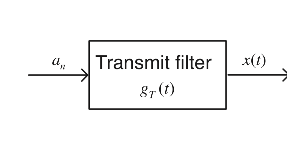
Let $x(t)$ essentially be a bunch of symbols ${a_n}$ that I choose to transmit at intervals $1/T$. We create $x(t)$ from these symbols by using a transmit filter $g(t)$.
ie…
$$x(t)= \sum_{m=-\infty}^{\infty} a_m g(t-mT)$$
We then operate this by the channel ($h(t)$) to get signal $y(t)$.
So,$y(t) = \sum_{m=-\infty}^{\infty} a_m h(t)*g_T(t-mT)$.
Again, on upon receiving, we encounter the receive filter and get:
$$y(t) = \sum_{m=-\infty}^{\infty} a_m g_R(t) * h(t)*g_T(t-mT)$$
In order to compensate for the channel, let’s add an equaliser $h^{-1}(t)$. Finally,
$$y(t) = \sum_{m=-\infty}^{\infty} a_m h^{-1}(t) * g_R(t) * h(t)*g_T(t-mT)$$
Or,
$$y(t) = \sum_{m=-\infty}^{\infty} a_m g_R(t) *g_T(t-mT) = \sum_{m=-\infty}^{\infty} a_m g(t-mT) $$
where, $g(t) = g_R * g_T$. In the preceeding section, we have just used the associative property of convolution.
This is conveniently seen as a block diagram.
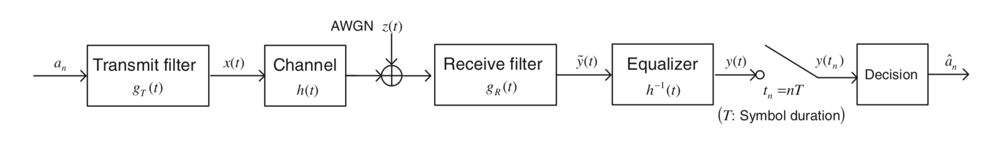
If we sample $y(t)$ at $t_n = nT$, we get:
$$y(t_n) = a_ng(0) + \sum_{m\neq n} a_m g((n-m)T)$$. Here comes our dilemma. Notice that we said $g(t)$ would be finite in Fourier domain, so it is infinite in time domain.
As a result, we cannot guarantee that, $g((n-m)T)= 0 \quad for n \neq m$. This causes the phenomenon of inter symbol interference (ISI).
ISI and the Nyquist Criterion
Assume we choose $g(nT) = \delta[n]$, hence, satisfying the previous requirement. This condition in the frequency domain equals,
$$\sum_{i=-\infty}^{\infty}G(f-\frac{i}{T})=T$$
This is the very well known Nyquist criterion.
One obvious candidate for this is the rectangle pulse, which looks like the graph below and is given by:
\begin{align*}
G_I(f) &= \frac{1}{2W}rect(\frac{f}{2W}) &= \left\{
\begin{array}{ll}
      T, \quad |f| \leq \frac{1}{2T}\\
      0, \quad \text{otherwise}\\
\end{array}
\right.
\end{align*}
import numpy as np
from matplotlib import pyplot as plt
%matplotlib inline

Fs = 100    # sampling frequency
T = 10      # time duration we want to look at
t = np.arange(-T, T, 1/Fs)  # the corresponding time samples

# define our two functions
x = lambda t: np.sinc(t) * np.hanning(len(t))

# the resulting time range, when convolving both signals

plt.figure(figsize=(10,4))
plt.subplot(121)
plt.plot(t, x(t))
plt.xlim(-6,6)
plt.grid()
plt.xlabel("Time")
plt.ylabel("Amplitude")
plt.title("Time domain")
plt.legend(("$x(t)$",))

plt.subplot(122)
# function to calculate the spectrum of the input signal
spec = lambda x: abs(np.fft.fftshift(np.fft.fft(x, 4*len(t))))/Fs
X = spec(x(t))
f = np.linspace(-Fs/2, Fs/2, len(X))
plt.plot(f, X)
plt.xlim(0,3)
plt.grid()
plt.legend(("$|X(f)|$",))
plt.xlabel("Normalised frequency")
plt.ylabel("Amplitude")
plt.title("Fourier domain")
plt.show()
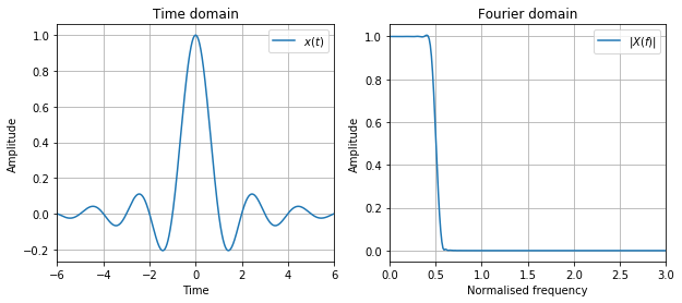
Unfortunately, we cannot realise the sinc function in practice due to its non causal nature, and as such resort to the following, called the raised cosine filter:
\begin{align*}
G_{RC}(f) = \left\{
\begin{array}{ll}
      T, \quad |f| \leq \frac{1-r}{2T}\\
      \frac{T}{2} (1 + \cos \frac{\pi T}{r} (|f| -\frac{1-r}{2T})), \quad \frac{1-r}{2T} \leq |f| \leq \frac{1+r}{2T} \\
      0, \quad \text{otherwise}\\
\end{array}
\right.
\end{align*}
As exercise 1, find the inverse fourier transform of the raised cosine filter (Hint: use numpy to plot it first and understand its analytical form. Then proceed backwards)
We controll the filter by its roll-off characteristics, $r$. Notice that as $r$ varies between 0 and 1, we move from an ideal low pass filter to a filter occupying twice the Nyquist bandwidth.
Now, we design for the receive and transmit filters, with the requirement that $G_R(f) = G_T^*(f)$. Thus,
\begin{align*}
G_{R}(f) = \left\{
\begin{array}{ll}
      \sqrt{T}, \quad |f| \leq \frac{1-r}{2T}\\
      \sqrt{\frac{T}{2} (1 + \cos \frac{\pi T}{r} (|f| -\frac{1-r}{2T}))}, \quad \frac{1-r}{2T} \leq |f| \leq \frac{1+r}{2T} \\
      0, \quad \text{otherwise}\\
\end{array}
\right.
\end{align*}
Notice that $GR(f)$ is not Nyquist, but $G{RC}(f)$ is. Is the converse true? That is if a filter satisfies the Nyquist criterion, does its square too? (exercise 2)
Limitations for High Data Rate
Thus, in order to transmit at rate $R_s$, we need to have a minimum bandwidth of $R_s/2$. Thus, with increasing data rate, we would need greater signal bandwidth.
If we cross the coherence bandwidth (see the earlier post on large scale fading), the equaliser no longer cancels out the channel effect (we incurr multi-path fading). Thus, we end up having ISI due to the multi-path fading.
In order to address this, we could try out adaptive equalisers. But can we do better?
Multiple Carrier Transmission
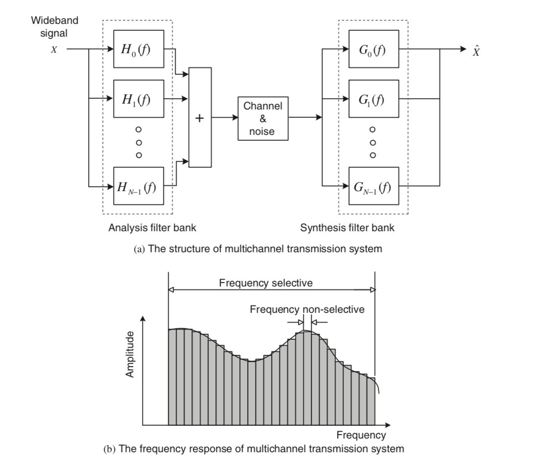
So here’s the idea, we transmit a wide band signal by splitting it up over mutliple frequency bins, each with channel transfer function $H_k(f)$, and multiple narrow band filters $G_k(f)$. Owing to the non-selectivity of each of these $H_k(f)$’s, we can equalise them.
Assuming these subcarriers are kept orthogonal, we will not have any Inter Channel Interference (ICI).
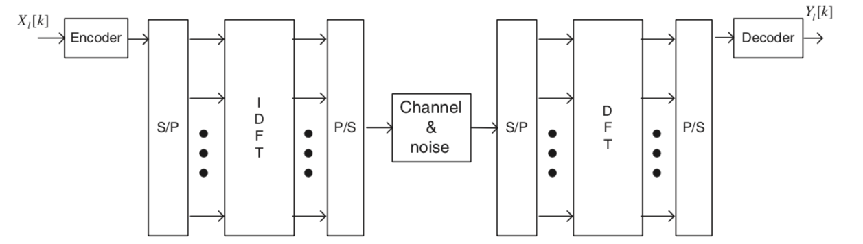
Assume $N$ narrowband subchannels, each with subcarrier frequency $f_k$. In essence, this is a form of Frequency Division Multiple Access (FDMA). The below two figures illustrate the general scheme.
OFDM
OFDM is one such FDMA system. Let $l$ denote the symbol interval, and consider the $k$ th frequency. Then we transmit $X_l[k]$ and receive $Y_l[k]$. Take the $N$ point IFFT of ${\{X_l[k]\}}_{k=0}^{N-1}$, to get $\{x[n]\}_{n=0}^{N-1}$.
From our previous post connecting FFT to Convolutions, we see that $x[n]$ are samples of the orthogonal signals sent in these $N$ channels.
Assume, we receive $y[n] = x[n] + w[n]$, where $w[n]$ is some white Gaussian noise (WGN, see the contents for a post on what WGNs are). And from $\{y[n]\}_{n=0}^{N-1}$, obtain via FFT $\{Y_l[k]\}_{k=0}^{N-1}$. Typically, we use rectangular pulses (of duration $T$) as subcarriers, thus the OFDM signal can be considered as the sum of the frequency shifted sinc functions (spaced by $1/T$ in the frequency domain as illustrated in the below figure.
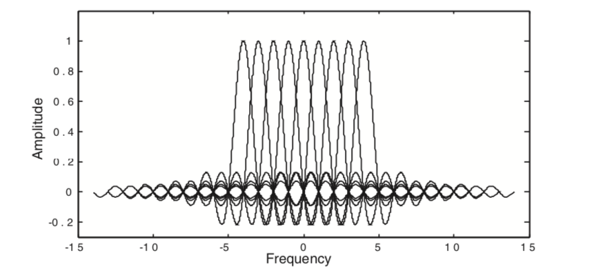
Notice that the first sidelobe is not so small as compared to the main lobe in the spectra, ie…, we are not dealing with bandlimited signals. This causes non-negligible adjacent channel interference (ACI), requiring guard bands and cyclic prefixes. We shall explain this in detail shortly.
OFDM Basics: Modulation and Demodulation
Consider the time-limited complex exponential signals $\exp(2j\pi f_k t)_{k=0}^{N-1}$ which represent the different subcarriers at $f_k = k/T_{sym}$ in the OFDM signal, where $0 \leq t \leq T_{sym}$. These signals are defined to be orthogonal if the integral of the products for their common (fundamental) period is zero. This is also known as their inner product, ie…,
$$<\exp(2j\pi f_k t), \exp(2j\pi f_i t)> := \frac{1}{T_{sym}}\int_0^{T_{sym}} \exp(2j\pi f_k t) \exp(-2j\pi f_i t dt = \delta_{k,i} $$, where $\delta_{k,i} = 1, k = i, 0$ otherwise is the Kronecker delta function.
An OFDM transmitter first converts seriel bits into parallel ($N$ parallel bits) via a S/P converter. Let $X_l[k]$ denote the $l \in {0,1,…,}$th transmit symbol at the $k \in {0,1,…,N-1}$ th subcarrier.
If $T_s$ is the duration of the subcarrier pulse, then the time to transmit the OFDM symbols would be $T_{sym} = NT_s$
Let’s transmit two different pieces of information $X_1,X_2$ using two different frequencies $f_1,f_2$:
$$\begin{align}x(t)&=X_1\exp(j2\pi f_1t) + X_2\exp(j2\pi f_2t)\\y(t)&=h(t)*x(t)=X_1\cdot H(f_1)\cdot\exp(j2\pi f_1t)+X_2\cdot H(f_2)\cdot\exp(j2\pi f_2t).\end{align}$$
Even more, let’s transmit not only two different pieces of information, but many. For each information, we use a different frequency, and denote the information on frequency $f$ by $X(f)$. Since we can transmit on any frequency, the transmit signal can be written as
$$x(t)=\int_{-\infty}^{\infty}X(f)\exp(j2\pi ft)df$$
For each frequency $f$, we transmit the information $X(f)$ on the complex exponential $\exp(j2\pi ft)$. You see, this is exactly the inverse Fourier Transform.
At the receiver side, the received signal becomes
$$y(t)=\int_{-\infty}^{\infty}X(f)H(f)\exp(j2\pi ft) df,$$
from which we actually want to obtain the amplitudes of the different frequency components $X(f)H(f)$. What do you do to obtain the information about the frequency components of a signal? Right, you perform Fourier Transform, which leads to
$$Y(f)=\mathcal{F}\{y(t)\}=X(f)H(f)$$
because $X(f)H(f)$ is the amplitude of the frequency component with frequency $f$.
What’s the problem with this approach? Well, the involved signals are infinitely long. So, in order to demodulate the signal, you’d need to wait infitinely long. Clearly, that’s not a practical solution.
Orthogonality of time-limited complex exponentials
What, if we do not want to wait infinitely long at the receiver, but only for a time period of length $T$? Hence, at the receiver we perform the Fourier Transform of a time-limited exponential, let’s say which ranges from $0$ to $T$. Hence, given a received signal of frequency $f_1$, by $x(t)=\exp(j2\pi f_1 t)$, what would be the result of the Fourier transform of this signal? Let’s use Sympy to do the tedious calculation:
import sympy as S
S.init_printing()
f1, f2, t, P = S.symbols("f1 f2 t P")
I = S.Integral(S.exp(2*S.I *S.pi*f1*t)*S.exp(-2*S.I*S.pi*f2*t), (t, 0, 1))  # write the integral
R = S.simplify(I.doit())  # calculate the integral
display(S.relational.Eq(S.relational.Eq(P(f1,f2), I), R))  # show the result
$$P{\left (f_{1},f_{2} \right )} = \int_{0}^{1} e^{2 i \pi f_{1} t} e^{- 2 i \pi f_{2} t}\, dt = \begin{cases} 1 & \text{for}\: f_{1} = f_{2} \\- \frac{i e^{- 2 i \pi f_{2}}}{2 \pi \left(f_{1} - f_{2}\right)} \left(e^{2 i \pi f_{1}} - e^{2 i \pi f_{2}}\right) & \text{otherwise} \end{cases}$$
The function does not look really nice. One could simplify it, but we dont care at this point. Let’s just plot it for different values of $f_1$ and $f_2$ and see what happens:
X = np.vectorize(lambda f1, f2: R.evalf(subs=dict(f1=f1,f2=f2)))
plt.figure(figsize=(6,2))
for f1 in (1, 2, 3, 4):
    f2 = np.linspace(0, 5, 100, endpoint=False)
    plt.plot(f2, abs(X(f1, f2)), label='$f_1=%d$' % f1)
plt.legend(fontsize=10); plt.grid(True); plt.xlabel('$f_2$'); plt.ylabel('$|P(f_1,f_2)|$');
plt.title("Interference from a signal with frequency $f_1$ onto the Fourier transform at frequency $f_2$.");
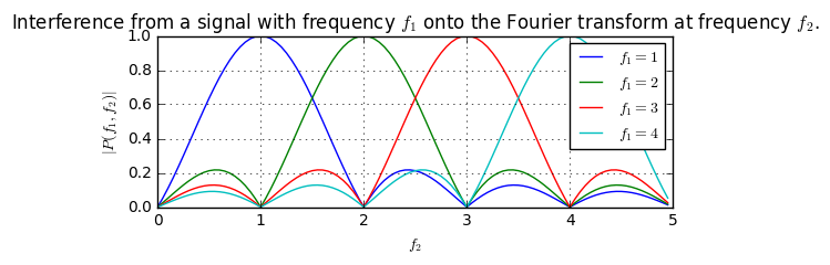
What does this figure show? It tells us, that if we transmit with a frequency of $f_1=1$ (blue curve), the output of the Fourier transform at frequencies $f_2={2,3,4,5,…}$ becomes $0$. Hence, the signal transmitted at frequency $f_1=1$ does not interfer with a signal that was transmitted at a frequency $f_2={2,3,4,5}$. These results hold for $T=1$. In general, it holds that $P(f_1,f_2)=0$ if $f_1-f_2=n/T$ with $n\in\mathbb{Z}$. (Essentially, what he have derived here is the Fourier transform of a rectangular function of length $T$.)
In conclusion, if we require that our receiver window should only be $T$ seconds long, we can only transmit signals at the frequencies $1/T, 2/T, 3/T, …$. The signals on these frequencies are called the OFDM subcarriers and this property ensures the orthogonality, i.e. it ensures that adjacent subcarriers do not interfer with each other after the Fourier transform at the receiver.
Influence of the wireless channel
Up to now, everything should be fine, right? We have shown that complex exponentials are orthogonal over a time period $T$, when their frequencies have a difference of $\Delta_f=f_1-f_2=n/T$ with $n\in\mathbb{Z}$. Furthermore, we have stated that complex exponentials are eigenfunctions of the channel, i.e. a transmitted complex exponential remains a complex exponential. So, problem solved?
No, unfortunately not. Only infinitely long complex exponentials are eigenfunctions of the channel. This means, if we transmit a complex exponential of length $T$, the output of the channel will not just be a scaling of the amplitude of this signal:
T = 1
t = np.arange(-1, 2, 1/Fs)
f1 = 20
x = np.cos(2*np.pi*f1*t) * (t>=0) * (t<1)
y = np.convolve(h, x)
y = y[:len(x)]

plt.subplot(121)
plt.plot(t, x)
plt.xlim((-0.1, 1.2)); plt.grid(True); plt.xlabel('$t [s]$'); plt.ylabel('$x(t)$'); plt.ylim((-1.1, 1.35)) # ilü
plt.annotate(s='',xy=(0,1.1), xytext=(1,1.1), arrowprops=dict(arrowstyle='<->'))
plt.text(0.5,1.1,r'Transmit interval $T$',va='bottom', ha='center', fontsize=12);
plt.title("Transmitted signal")

plt.subplot(122)
plt.plot(t, y)
plt.xlim((-0.1, 1.2)); plt.grid(True); plt.xlabel('$t [s]$'); plt.ylabel('$y(t)=h(t)*x(t)$'); plt.ylim((-8.5, 8.5))
plt.annotate(s='',xy=(0,6.7), xytext=(1,6.7), arrowprops=dict(arrowstyle='<->'))
plt.text(0.5,6.7,r'Receive interval $T$',va='bottom', ha='center', fontsize=12);
plt.title("Received signal after multipath channel")
plt.tight_layout()
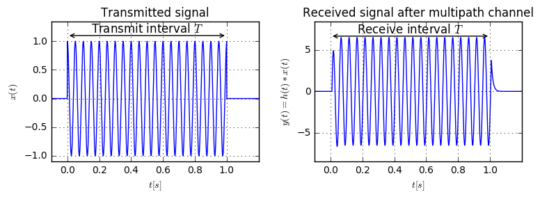
Apparently, at the beginning of the received interval, the signal is severely distorted. This would lead to a non-accurate signal reception. Hence, this technique is not applicable in a multpath channel. What can we do?
Even though it looks like the signal is also distorted at the end of receive interval, this is not the case: The channel introduces a delay to the harmonic function, shifting the wave slightly to the right, hence the wave won’t reach its maximum at $t=1$. This is due to the phase delay of the channel.
The Necessity of the Cyclic Prefix
We know the received signal is the convolution of the channel’s impulse response with the transmitted signal and only infinitely long complex exponentials are eigenfunctions of the channel. But, we want to have time-limited complex exponentials at the output of the channel.
Knowing that the channel impulse response has length $L$, we know that the channel output at time $t_0$ does only depend on the channel input at times $t_0-L\leq t\leq t_0$, i.e. the channel does have a limited memory, it can only remember the last $L$ seconds of the input signal. Consequently, the channel does not care, if the input signal is an infinitely long complex exponential or not, it only cares about the last $L$ seconds of the signal. Therefore, we can trick the channel by transmitting a complex exponential of length $T+L$, and the channel will output a perfect complex exponential during the times $L\leq t\leq T+L$:
L = 0.1 # the channel length
x = np.cos(2*np.pi*f1*t) * (t>=-L) * (t<T)
y = np.convolve(h, x)[:len(x)]

plt.subplot(121)
plt.plot(t, x)
plt.xlim((-0.2, 1.2)); plt.grid(True); plt.xlabel('$t [s]$'); plt.ylabel('$x(t)$'); plt.ylim((-1.1, 1.35))
plt.annotate(s='',xy=(-L,1.1), xytext=(1,1.1), arrowprops=dict(arrowstyle='<->'))
plt.text(0.5-L/2,1.1,r'Transmit interval $T+L$',va='bottom', ha='center', fontsize=12);
plt.title("Transmitted signal")

plt.subplot(122)
plt.plot(t, y)
plt.xlim((-0.2, 1.2)); plt.grid(True); plt.xlabel('$t [s]$'); plt.ylabel('$y(t)=h(t)*x(t)$'); plt.ylim((-8.5, 8.5))
plt.annotate(s='',xy=(0,6.7), xytext=(1,6.7), arrowprops=dict(arrowstyle='<->'))
plt.text(0.5,6.7,r'Receive interval $T$',va='bottom', ha='center', fontsize=12);
plt.title("Received signal after multipath channel")
plt.tight_layout()
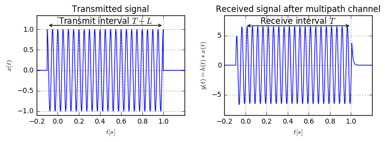
As we see, now the distortion of the transmitted signal occurs outside of the receiver interval. Within the receiver interval the waves are perfect. Hence, within this interval our orthogonality condition holds and we can detect our data without interference.
You might have already guessed that the extra part at the beginning of the block is called the Cyclic prefix. Some people call it guard interval, which seems more appropriate to our current application: It guards the actual receiver interval such that it contains a perfect harmonic function. Why is it also called Cyclic prefix? We know that the complex exponentials with frequencies $1/T, 2/T, \dots$ are periodic with period $T$. Therefore, the we have $x(t-T)=x(t)$, which shows that the guard interval is actually a copy of the end of the block. Therefore, it’s called cyclic prefix (CP), because the CP creates a cyclic block structure by prepneding the end of the block to its beginning.
References
- MIMO OFDM Wireless Communications, Y. Chang and W. Yang, IEEE Press, 2010.
- Sympy Docs.
- Numpy Docs.