Introduction to Communication Systems
In recent years, we’ve come to take multiple facets of technology for granted. It is normal to expect a light to spontaneously turn on when the switch is flipped; just as it’s normal to be able to watch and read news reports on a smartphone. The reach of the information age has deepened in the country, and more people now have access to a wealth of knowledge and opinions. This process of information transfer, either through space or time (think storage) is what we’ll call communication. From cellular phones to satellites, communication technology has revolutionised the world we live in. Industry, education, and governance have benefitted from the world drawing closer together. This very course itself is an example of something that would not have been possible without advances in communication systems :). Even today, researchers are looking at improving these systems. From improving data rates to connecting millions of devices, there’s a lot of problems to be solved in the domain.
A Brief History
Adapted from Wikipedia: The Free Encyclopedia
The idea of wireless communication predates the discovery of “radio” with experiments in “wireless telegraphy” via inductive and capacitive induction and transmission through the ground, water, and even train tracks from the 1830s on. James Clerk Maxwell showed in theoretical and mathematical form in 1864 that electromagnetic waves could propagate through free space. It is likely that the first intentional transmission of a signal by means of electromagnetic waves was performed in an experiment by David Edward Hughes around 1880, although this was considered to be induction at the time. In 1888 Heinrich Rudolf Hertz was able to conclusively prove transmitted airborne electromagnetic waves in an experiment confirming Maxwell’s theory of electromagnetism.
After the discovery of these “Hertzian waves” (it would take almost 20 years for the term “radio” to be universally adopted for this type of electromagnetic radiation) many scientists and inventors experimented with wireless transmission, some trying to develop a system of communication, some intentionally using these new Hertzian waves, some not. Maxwell’s theory showing that light and Hertzian electromagnetic waves were the same phenomenon at different wavelengths led “Maxwellian” scientist such as John Perry, Frederick Thomas Trouton and Alexander Trotter to assume they would be analogous to optical signaling and the Serbian American engineer Nikola Tesla to consider them relatively useless for communication since “light” could not transmit further than line of sight. In 1892 the physicist William Crookes wrote on the possibilities of wireless telegraphy based on Hertzian waves[8] and in 1893 Tesla proposed a system for transmitting intelligence and wireless power using the earth as the medium. Others, such as Amos Dolbear, Sir Oliver Lodge, Reginald Fessenden, and Alexander Popov were involved in the development of components and theory involved with the transmission and reception of airborne electromagnetic waves for their own theoretical work or as a potential means of communication.
Over several years starting in 1894 the Italian inventor Guglielmo Marconi built the first complete, commercially successful wireless telegraphy system based on airborne Hertzian waves (radio transmission). Marconi demonstrated the application of radio in military and marine communications and started a company for the development and propagation of radio communication services and equipment.
#TODO: Add a graphic (from Prof. David's slides possibly) of evolving radio technology over the years till date.
Analog and Digital Communication
Radio waves can be artificially generated, and they propagate through free space. The natural response to this discovery is to explore whether we can manipulate these waves to enable useful applications. In the case of communication, we would like to encode information onto these radio waves in some manner. For example: turning the radio wave on and off is a way by which we can signal a change in state. As you might have guessed, there must be much more efficient ways to encode information onto radio waves, and there are. By manipulating the amplitude and phase of radio waves in a deterministic manner, we can map complicated messages onto a radio wave at the transmitter and reliably decode the message at the receiver. This technique of mapping a message signal onto a radio wave is broadly referred to as modulation.
While we have been mostly concerned with radio waves, the concepts discussed in this module apply generally to any communication technique using waves that propogate in a medium (like sound waves in the sea). Wireless communication majorly deals with smartly engineering transceiver systems that operate in a given wireless channel (the medium that the radio wave propogates in).
There are two major classes in wireless communication: analog and digital. The initial use of wireless communication was to send speech and audio signals over long distances. One can understand intuitively that these signals represent some useful information. These are message signals that we want to use our communication system to convey. All signals in nature are continuous time signals, i.e they are analog in nature. Even if voice is recorded in a digital storage medium like a hard drive, it is still consumed as an analog signal through the speaker. Radio waves (electromagnetic waves) are also analog in nature.
- Analog Communication: Given that many message signals and the communication signal (radio waves) are analog in nature, it makes sense to map analog message signals directly onto analog communication signals. This is what is done in AM (Amplitude Modulation), FM (Frequency Modulation), first generation cell phone technology and vinyl records. While this seems natural for voice and music, analog communication is now obsolete. In many situations, it has been replaced with its digital counterpart. For example, current cellular phone technology, compact disks and digital satellite TV are all based on digital communication.
Digital Communication: The basis of this field was established in a seminal paper by Claude Shannon in 1948. There are two major tenets in Shannon’s work: Source Coding (& Compression) and Digital Information Transfer (aka. channel capacity). Shannon showed that any information-bearing signal can be represented efficiently (with required precision of reproduction)0
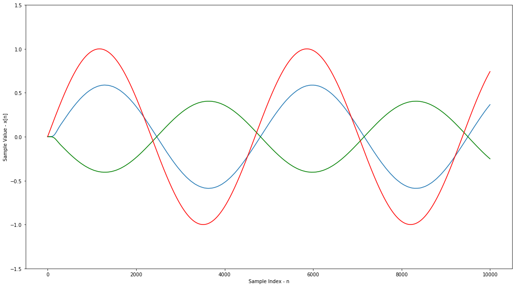
%matplotlib inline
import numpy as np
import matplotlib.pyplot as plt
from scipy import signal
t = np.arange(0,1,0.0001); # Sampling time instants x_c = np.sin(2*np.pi*100*t); x_c_2 = np.sin(2*np.pi*100*t+0.3*np.pi); x_d = np.cos(2*np.pi*100*t+0.3*np.pi); x = np.sin(2*np.pi*2.1332*t); x_p = x*x_c x_b_q = x_p*x_c_2 x_b_i = x_p*x_d b, a = signal.butter(6, 0.01, btype='low', analog = False); x_b_i = signal.lfilter(b,a,x_b_i); x_b_q = signal.lfilter(b,a,x_b_q); fig=plt.figure(figsize=(18, 10), dpi= 80, facecolor='w', edgecolor='k') plt.plot(2*x_b_q) plt.plot(x_b_i,'g') plt.plot(x,'r') plt.xlabel('Sample Index - n') plt.ylabel('Sample Value - x[n]') plt.ylim([-1.5,1.5]); plt.show()
help(signal.lfiltic)
Help on function lfiltic in module scipy.signal.signaltools:

lfiltic(b, a, y, x=None)
    Construct initial conditions for lfilter.

    Given a linear filter (b, a) and initial conditions on the output `y`
    and the input `x`, return the inital conditions on the state vector zi
    which is used by `lfilter` to generate the output given the input.

    Parameters
    ----------
    b : array_like
        Linear filter term.
    a : array_like
        Linear filter term.
    y : array_like
        Initial conditions.

        If ``N=len(a) - 1``, then ``y = {y[-1], y[-2], ..., y[-N]}``.

        If `y` is too short, it is padded with zeros.
    x : array_like, optional
        Initial conditions.

        If ``M=len(b) - 1``, then ``x = {x[-1], x[-2], ..., x[-M]}``.

        If `x` is not given, its initial conditions are assumed zero.

        If `x` is too short, it is padded with zeros.

    Returns
    -------
    zi : ndarray
        The state vector ``zi``.
        ``zi = {z_0[-1], z_1[-1], ..., z_K-1[-1]}``, where ``K = max(M,N)``.

    See Also
    --------
    lfilter